4.2 - Alpha Structures Implementation

As previously said in section 3.3 we have addressed the problem of evaluate $\alpha$-structures via $\alpha$-filtering evaluation (namely the evaluation of the characteristical $\alpha$ for each simplex).

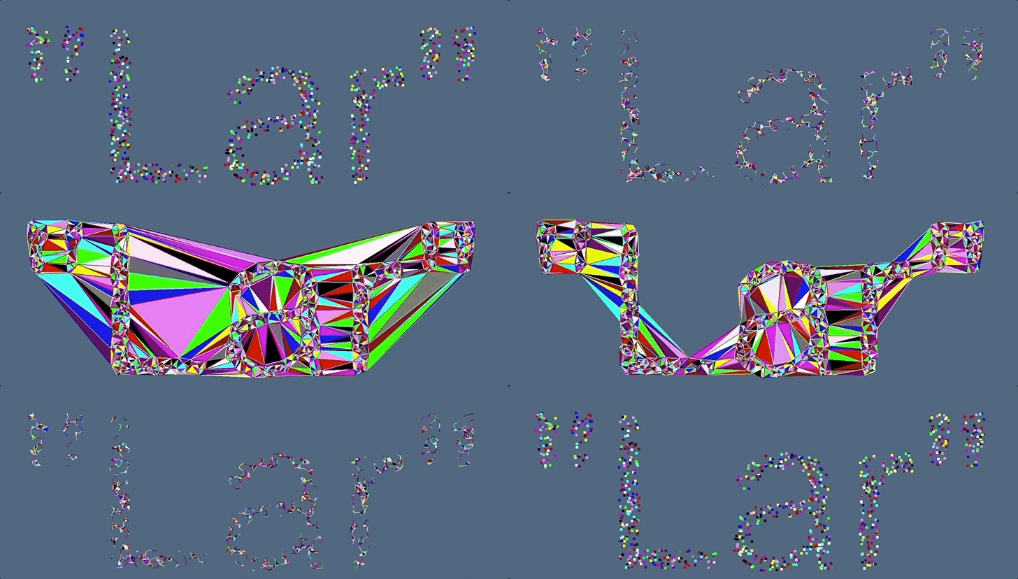
Figure 1: 2D Alpha Shape with various $\alpha$

The tasks

We could decompose the problem into three tasks:

• evaluate the triangulation decomposition of the Sites $S$
• evaluate the characteristical $\alpha$
• sort the simplices according to their $\alpha$.

The first task to solve is to evaluate the Triangulation. However we have discussed this problem in the previous section.

The last task also is pretty simple and teherefore we will not talk about it in this context.

The second task is the hardest to achieve. It is pretty clear that each site $s \in S$ has a characteristical $\alpha$ equal to zero. The real problem occurs then when we want to evaluate the characteristical $\alpha$ of all the other simplices.

Evaluate Characteristical $\alpha$

In order to obtain a simple method to evaluate characteristical $\alpha$ so that it is dimensional indipendent we could use the dual of the Delaunay Triangulation we have described in section 3.2: the Voronoy Diagram.

In fact the following relation occurs:

To simplify this notion we could refer to what happend in the two dimensional case:

Of course we could overturn the point of view by looking what happend if we consider the $d-1$-dimensional ball $\mathcal B$ centered in the center of the circumball defined by the $d$ sites of $\sigma$. First of all we are sure it is well defined and unique since $S$ satisfies the general position condition. The stated condition then assume the following form:

In particular the last statement implies that the characteristical $\alpha$ of a simplex $\sigma$ is always bigger or equal than the circumradius of the sites it is made of. Moreover for usual conditions (namely no higher dimensional obtuse-solid-angled simplices) the characteristical $\alpha$ is precisely that value.

This key feature is the one we have used in our implementation. In fact, the problem of determine if a simplex is (or is not) obtuse-angled is pretty simple. It suffices to determine if its circumcentre is (or is not, respectivelly) located outside the simplex itself.

The Pipeline

The approach we have followed could be summed up into the following pipeline:

1. Delaunay triangulation of the Sites $S$ (highest degree simplices)
2. Construction of lower degree simplices via Combinatorics.combinations()
3. Evaluation of Circumballs Radius for each simplex
4. Evaluation of the Characteristical $\alpha$ for each simplex
5. Sorting the simplices by their $\alpha$ in a DataStructures.SortedMultiDict

Example

julia> using AlphaStructures, ViewerGL

julia> GL = ViewerGL

julia> V = [
 0.52 0.61 0.71 0.55 0.81 0.20 0.01 0.54 0.54 0.96 0.35 0.42 0.55 0.92 0.41 0.36 0.23 0.35 0.11 0.59
 0.38 0.47 0.17 0.91 0.62 0.06 0.54 0.20 0.96 0.27 0.07 0.03 0.05 0.57 0.14 0.65 0.05 0.27 0.62 0.53
];

julia> filtration = AlphaStructures.alphaFilter(V);
SortedMultiDict(Base.Order.ForwardOrdering(),
    0.0 => [1], 0.0 => [2], 0.0 => [3]  …
    0.8948905417047672 => [10, 13], 0.8948905417047672 => [3, 10, 13]
)

julia> VV,EV,FV = AlphaStructures.alphaSimplex(V,filtration,0.25)
3-element Array{Array{Array{Int64,1},1},1}:
 [[1], [2], [3]  …  [18], [19], [20]]

 [[1, 2], [1, 3], [1, 8]  …  [16, 20], [17, 18], [18, 19]]  

 [[1, 2, 3], [1, 2, 20], [1, 3, 8]  …  [11, 17, 18], [12, 13, 15], [16, 18, 19]]

julia> points = [[p] for p in VV];

julia> faces = [[f] for f in FV];

julia> edges = [[e] for e in EV];

julia> GL.VIEW( GL.GLExplode(V, [points; edges; faces], 1.5, 1.5, 1.5, 99, 1) );

Main Interface

The solution we have proposed is located in the alphaFilter function (in this file):

alphaFilter(
	V::Matrix, DT = Array{Int64,1}[];
	digits=64
)::DataStructures.SortedMultiDict{}

julia> V = [1. 2. 1. 2.; 0. 0. 1. 2. ];

julia> AlphaStructures.alphaFilter(V)
SortedMultiDict(Base.Order.ForwardOrdering(),
	0.0 => [1],
	0.0 => [2],
	0.0 => [3],
	0.0 => [4],
	0.5 => [1, 2],
	0.5 => [1, 3],
	0.70710678118655 => [2, 3],
	0.70710678118655 => [3, 4],
	0.70710678118655 => [1, 2, 3],
	1.0 => [2, 4],
	1.0 => [2, 3, 4]
)

alphaSimplex(
	V::Matrix,
	filtration::DataStructures.SortedMultiDict{},
	α_threshold::Float64
)::Array{Array{Array{Int64,1},1},1}

delaunayTriangulation(V::Matrix)::Array{Array{Int64,1},1}

julia> V = [1. 2. 5. 6. 0. 7.];

julia> DT = AlphaStructures.delaunayTriangulation(V)
5-element Array{Array{Int64,1},1}:
 [1, 5]
 [1, 2]
 [2, 3]
 [3, 4]
 [4, 6]

julia> V = [
 1. 2. 1. 2. ;
 0. 0. 1. 2.
];

julia> DT = AlphaStructures.delaunayTriangulation(V)
2-element Array{Array{Int64,1},1}:
 [1, 2, 3]
 [2, 3, 4]

julia> V = [
 1. 2. 1. 2. ;
 0. 0. 1. 2. ;
 3. 1. 0. 2.
];

julia> DT = AlphaStructures.delaunayTriangulation(V)
1-element Array{Array{Int64,1},1}:
 [1, 2, 3, 4]